Create Pivot Table in Excel
Knowing the steps to create Pivot Table in Excel will make you far more productive, compared to using TOTAL, SUBTOTAL and other commands to analyze Data. The first step in creating an error free Pivot Table is to make sure that the Source Data for Pivot Table is in the right format. Once the Source Data is ready, you can either insert a blank pivot table or insert one of the suggested PivotTables into the worksheet. In our opinion, going with a Suggested Pivot Table and modifying it is easier and quicker than working with a blank Pivot Table.
1. Prepare Source Data For Pivot Table
In general, the Source data for Pivot Table needs to comply with the following requirements
- Each and every column in Source Data needs to have a heading or column Label. To avoid confusion, column Labels need to be unique and not repeated.
- Source Data cannot have blank columns. In-fact, you won’t be able to Create Pivot Table, if there is blank Column in the Source Data.
- Avoid blank Cells and blank Rows in Source Data, as they can lead to errors and confusion in Pivot Table.
- Do not include Totals, Subtotals and Averages (Column or Row Totals) when you select Source Data Range in a Pivot Table.
- Make sure that you apply formatting (Date, Number, etc.) to cells within the Source Data. Once the Source Data for Pivot Table is properly organized and meets the above requirements, you should have no problem creating error free Pivot Tables.
2. Insert Pivot Table into Worksheet
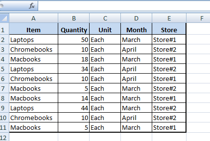
To explain the basic steps to Create Pivot Table in Excel, we will be making use of Sales Data recorded at two computer stores, conveniently labelled as Store#1 and Store#2.
As you can see in above image, the Source Data is well organized with unique column labels and it has no blank columns, blank rows or cells. Once the Source Data is in the right-format, you can follow the steps below to Create Pivot Table in Excel.
Open the Excel File containing Source Data that you want to include in the Pivot Table.
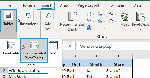
Select any Cell in Source Data > click on Insert > Tables > Recommended PivotTables option.
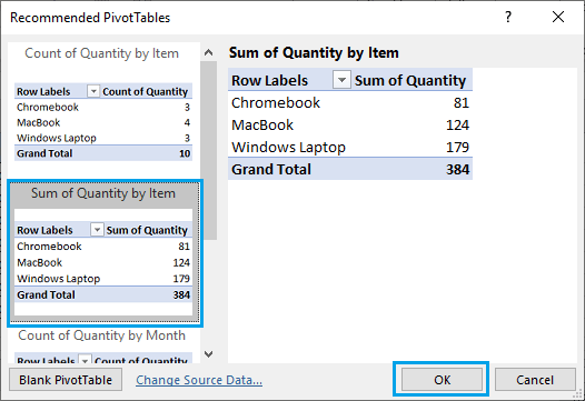
On Recommended PivotTables screen, scroll down the suggested list to view them > select the PivotTable Layout that you want to use and click on OK.
Note: You can actually click on the suggested PivotTable Layouts to see them in larger view. A layout will not be inserted, until you click on the OK button. 4. Once you click on OK, Excel will insert a Pivot Table in a new worksheet.
3. Modify Pivot Table Layout
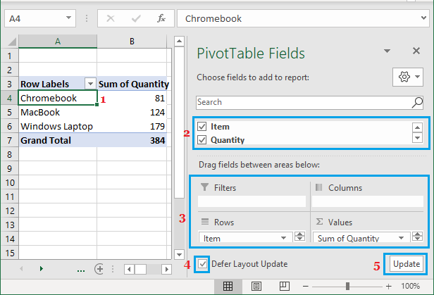
Even after creating PivotTable using the suggested layout, you can modify the PivotTable to suit your own requirements. Click on any Cell within the Pivot Table and this will open the PivotTable Field List.
Once the PivotTable Fields list is active, you will be able to modify the Pivot Table by adding Field Items and dragging the Field Items between Columns, Rows and Values areas. At first, you may find things going horribly wrong when you try to modify the Pivot Table layout. However, the only way to master Pivot Tables is to play around and make mistakes. It is recommended that you spend quality time to play around with PivotTable Field items and get used to modifying a given Pivot Table. Once you get familiar with modifying Pivot Table, you will be able to analyze large amounts of data and create all kinds of data summaries with effortless ease.
How to Change Pivot Table Data Source and Range How to Add or Remove Subtotals in Pivot Table How to Automatically Refresh Pivot Table Data